Forward modeling examples

Two example cases ship under examples/. Both are forward-modeling cases.

Canonical marine CSEM model

examples/canonical_model is a marine CSEM benchmark: a thin, resistive layer buried in conductive sediments beneath a seawater column. It exercises the full forward workflow (preprocess → fm.csem → postprocess) and is validated against a precomputed reference.

Model

Four layered materials, each a Gmsh physical volume in mesh.geo:

Layer	Volume tag	Depth z (m)	Conductivity
Water	4	0 … -1000	3.3333 S/m
Sediments 1	3	-1000 … -2000	1.0 S/m
Oil (target)	2	-2000 … -2100	0.01 S/m
Sediments 2	1	-2100 … -3500	1.0 S/m

The 100 m-thick Oil layer is the resistive target, about 1 km below the seafloor. Row i of sigmas.txt corresponds to physical tag i + 1.

Acquisition:

• Frequency: 2 Hz.

• Source: one x-directed horizontal electric dipole at (1750, 1750, -975) m (25 m above the seafloor), unit current and length.

• Receivers: an inline seafloor profile of 58 receivers at z = -990 m, y = 1750 m (receivers.txt).

Running

make

export MODEL_DIR=examples/canonical_model
export ORDER=1

# 1. Mesh generation
gmsh -3 ${MODEL_DIR}/mesh.geo -o ${MODEL_DIR}/mesh.msh

# 2. Input bundle + parameter file
python3 utils/preprocess.py \
   -mode fm \
   -order ${ORDER} \
   -case_dir ${MODEL_DIR} \
   -mesh_filename mesh.msh \
   -source_filename sources.txt \
   -receiver_filename receivers.txt \
   -sigma_file sigmas.txt \
   -input_filename input_p${ORDER}.h5 \
   -params_filename params_p${ORDER}.txt \
   -output_vtk model.vtu

# 3. Forward modeling
mpirun -n 4 build/fm.csem \
   -options_file ${MODEL_DIR}/params_p${ORDER}.txt

# 4. Compare against the reference
python3 ${MODEL_DIR}/postprocess.py \
   -case_dir ${MODEL_DIR} \
   -input_filename input_p${ORDER}.h5 \
   -responses_filename responses_p${ORDER}.h5 \
   -reference_filename reference.h5 \
   -figure_filename fields_p${ORDER}.png \
   -tolerance 0.03

Steps in detail:

1. Mesh generation. mesh.geo is a parametric Gmsh script (layers, plus refinement along the source/receiver line); gmsh -3 produces the tetrahedral mesh.msh.

2. Preprocessing. utils/preprocess.py -mode fm assembles the input bundle from the mesh, conductivity table, receivers, and sources, and emits the matching parameter file. -output_vtk additionally writes the conductivity model for visualization.

3. Forward modeling. fm.csem computes the responses and writes them to responses_p${ORDER}.h5 under -output_dir.

4. Validation. postprocess.py compares \(|E_x|\) against reference.h5, reports the NRMSD, relative L2, and MAPE, writes a comparison figure, and exits non-zero if the NRMSD exceeds -tolerance (default 0.03).

Other polynomial orders

The case ships a single mesh.geo. To run another order, either regenerate the bundle with a different -order, or override it at run time - which bypasses the bundle’s stored value:

mpirun -n 4 build/fm.csem \
   -options_file ${MODEL_DIR}/params_p1.txt -order 2 \
   -output_filename responses_p2

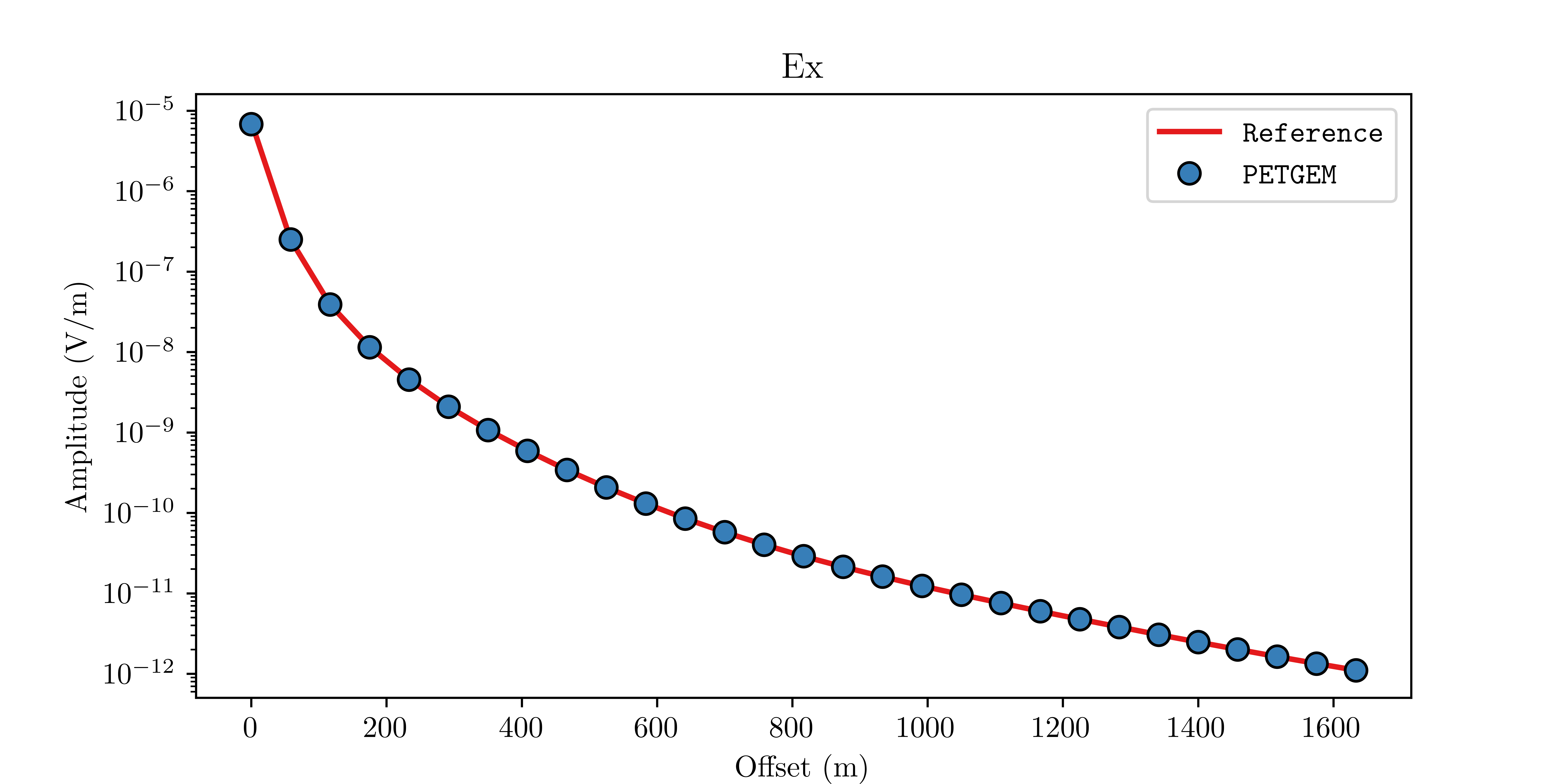
Comparison of the electric field component \(E_x\) between PETGEM and the reference solution.

Unit cube

examples/unit_cube is a homogeneous unit cube (\(\sigma = 1\) S/m) with one 2 Hz dipole at the centre and three receivers. It is the dataset the test suite is built around (see Testing), small enough to run the full pipeline for several orders in CI.

Its input.h5 and params_p1.txt are generated artifacts, rebuilt from the committed mesh.geo and *.txt inputs with the same workflow as above:

gmsh -3 examples/unit_cube/mesh.geo -o examples/unit_cube/mesh.msh
python3 utils/preprocess.py -mode fm -order 1 \
    -case_dir examples/unit_cube -mesh_filename mesh.msh \
    -source_filename sources.txt -receiver_filename receivers.txt \
    -sigma_file sigmas.txt -params_filename params_p1.txt

The mesh is structured (transfinite), hence reproducible across Gmsh versions. Committed reference responses for orders 1-3 live in examples/unit_cube/reference/.

Extrae profiling

fm.csem can be built with Extrae instrumentation to produce execution traces for Paraver. The Extrae configuration (extrae.xml, petgem_labels.txt, and the Paraver configuration petgem_functions.cfg) lives under tests/extrae/; the run below uses the unit_cube bundle, and is the same execution exercised in CI.

# Build with instrumentation -> build/fm.csem.extrae
make USE_EXTRAE=1

export LD_LIBRARY_PATH=${EXTRAE_HOME}/lib:$LD_LIBRARY_PATH
export EXTRAE_CONFIG_FILE=$PWD/tests/extrae/extrae.xml

mpirun -n 4 build/fm.csem.extrae \
    -input_filename examples/unit_cube/input.h5 \
    -order 1 -output_dir . -output_filename extrae_smoke

# Merge the intermediate files into a Paraver trace
${EXTRAE_HOME}/bin/mpi2prv -f TRACE.mpits -o petgem.prv

Extrae writes its intermediate TRACE.* files into the current working directory. The resulting petgem.prv opens in Paraver with tests/extrae/petgem_functions.cfg.

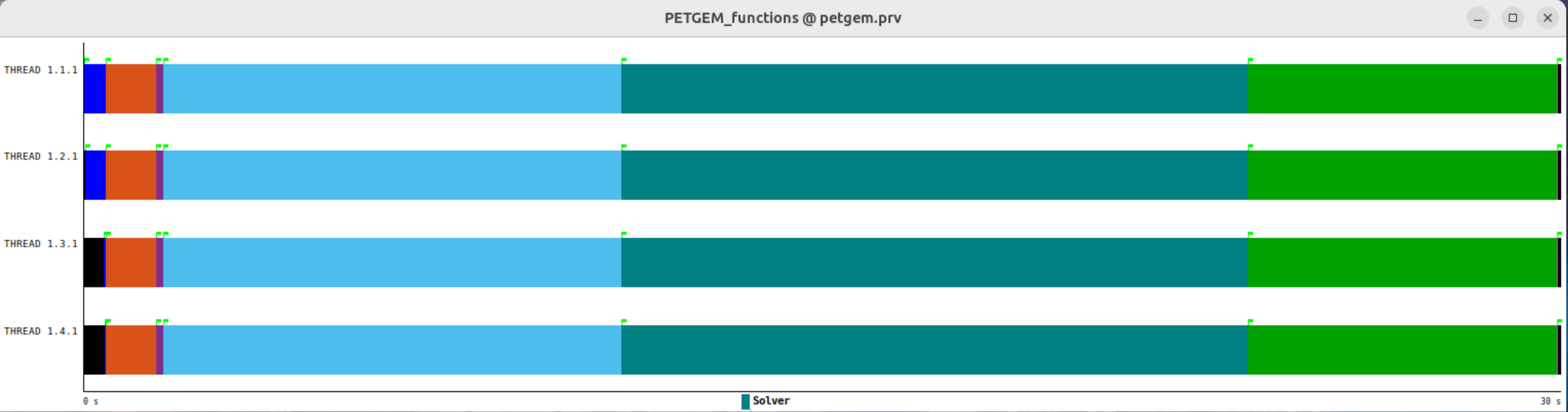
Extrae trace of a PETGEM simulation executed with 4 MPI tasks. Each color is an instrumented phase of the execution.